Smooth Out the Noise of Daily Data With Moving Averages in SQL

The moving average is the Swiss Army knife of metrics. It's adaptable, reliable, and simple to use.

Stock traders know this better than anyone. They modify the moving average calculation in a ton of different ways depending on what they want to know. Here are just a few applications:

• To confirm a trend. Traders use a simple moving average to establish a trend that can be used as a baseline to see if the stock price is trending up or down. To put emphasis on recent information, some traders will swap out the simple moving average, which gives the same weight to all data points, for an exponential moving average, which gives more weight to the newest data points.
• To measure a stock's momentum. Traders commonly calculate moving averages over three time periods: 20 days or less, 20 to 100 days, and 100 days or more. Using varying time frames like this allows them to compare the short-, medium-, and long-term price movements.
• To determine price supports. Traders use the moving average to determine how low the stock price will go before it bounces back up—this is called a support. Often, a stock price will fall and then rebound off the moving average and rise again. Traders can then set up a stop-loss order so they won't lose more money when the price falls below the moving average.

The moving average is really effective when you're working with data that's continuously updated. It moves along with the dataset (hence the name), dropping the oldest data points and adding new ones. This ensures that you're seeing the most recent trend, and not the trend since you first started gathering data.

No matter how you're using them, moving averages always accomplish one thing: they smooth out noise caused by fluctuations in your data so you can spot overall trends.

But investors don't have a monopoly on the moving average. Like stock prices, startup metrics such as engagement, signups, and sales change day-to-day, making moving averages handy for business analysts who want to track the overall trend of their growth (hopefully it's going up and to the right!).

Using moving averages to measure user engagement

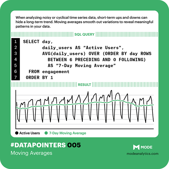
Smooth out those peaks and valleys with the Swiss Army knife of metrics! Check out our other #datapointers here.

At Mode, we use a simple seven-day moving average when reviewing engagement data. Before diving into calculating moving averages in SQL, let's take look at the raw data. To do that, we'll use this query of sample data:

SELECT day AS "Day",
   	   users AS "Active Users”
  FROM engagement
 ORDER BY day DESC

See the trough every Saturday and Sunday? Yep—it's pretty obvious. Since this sample data mimics that of a B2B SaaS company, the weekend dips are expected. As long as the numbers come back up each Monday, there's no cause for concern.

Did you also notice the small drop in active users in the last three weeks? All that noise makes it tricky to pick it out. But it's the pattern we need to see. If we fail to catch the trend, we're not going to ask why engagement is down—and we're not going to take steps toward deeper analysis. And that's a problem.

To smooth out the weekend dips and better see the downward trend, we can calculate a seven-day moving average using a windowing function in SQL. The table below shows the daily active users over a two-week period, starting on a Sunday (August 17, 2014).

The moving average basically says: take the count for any given day and the counts for each of the six preceding days, and average them all together. So, the calculation for the moving average for August 30 includes the active user counts from Sunday, August 24 to Sunday, August 30.

(65+285+284+298+339+305+149)/7 = 246.43

That means that over the last seven days, there was an average of 246.43 daily active users on the site. This can be applied to the data in the graph above by running this query:

SELECT day AS "Day",
   	   users AS "Active Users",
       AVG(users) OVER (ORDER BY day ROWS BETWEEN 6 PRECEDING AND 0 FOLLOWING)::FLOAT AS "7-Day Moving Average"
  FROM engagement
 ORDER BY 1 DESC

Which produces this graph (with the smoothed time trend in orange):

The key to it all is this line:

AVG(users) OVER (ORDER BY day ROWS BETWEEN 6 PRECEDING AND 0 FOLLOWING)

Let’s break this down:

• AVG() specifies the function that will be called over a specific column (in this case, daily_signups).
• OVER contains two pieces of information: 1) ORDER BY orders our rows based on the values of day. 2) ROWS BETWEEN 6 PRECEDING AND 0 FOLLOWING indicates that for every individual day, the average value of users will be taken for that day and the six days immediately preceding it.
• ::FLOAT ensures that this column of data is cast as numeric. Otherwise the data won't appear in the line chart because the system thinks it's text, not numbers. This is a problem with windowing functions similar to the FORMAT function in Excel.

With the dips smoothed out, it's easier to see that the number of daily active users declined from about 290 to about 240 over the last three weeks. This trend could be a cause for concern—or at the very least a place to focus optimization efforts and experiments to increase user engagement. With this knowledge in hand, we can move onto figuring out what caused the decline and how to fix it.

Modifying the time frame

We use a seven-day moving average at Mode because it lets us see changes in engagement quickly, but you can use any time period that's applicable to your business or problem at hand. Simply change the numbers in ROWS BETWEEN 6 PRECEDING AND 0 FOLLOWING to reflect your preferred time frame. If you want to learn more about the pros and cons of increasing the time frame for a moving average, here's a technical explanation.

That exponential moving average that stock traders use? That's doable in Mode, too. Check out this T-SQL blog post by Tomas Lind.

Ready to try out moving averages yourself? Try writing these queries against sample data in the public data warehouse data sets. Or, connect your database and start exploring trends in your own user data!